WHI index page (10.13.2004/01.01.2008)
homepage
WHI MORTALITY RATES
New Analysis by

Timothy D. Bilash MD MS OBGYN
www.DrTimDelivers.com
October 27, 2004
Lower Mortality? with Continuous Estrogen-Progestin
in the
Women's Health Initiative Menopause Study (2002)
sponsored by the U.S. Government National Institutes of Health
An alternative statistical approach applied to the
Women's Health Initiative Estrogen+Progestin Study shows a decreasing Mortality Rate with Continuous Prempro (EP)
over time compared to Placebo (PL),
which is contrary to the published report.
The simple linear model, although limited, provides insight into the
possibility that data anomaly (in Outcome Year4 specifically)
decreases the power of the published study findings to find an effect of Estrogen+Progestin on mortality.
This poster was presented at the
North American Medical Society Annual Meeting (October 6-9, 2004)
[Menopause 2004;11(6):664(P-43)]
Additional plots of the Cox WHI Annualized Mortality Rates and Change in %Censored Patients graphs have been added to this web version. Rates are shown as percent (with a decimal point) or per 100,000 (no decimal point).
Statistical calculations were coded and graphing was done in Appleworks6 (Apple) or Excel98 (Microsoft).

P43 ABSTRACT

Time Dependence of Mortality Rates in the Estrogen Plus Progestin Hormone Replacement Women's Health Initiative (WHI) Study

Timothy D Bilash, MD MS
North American Menopause Society (NAMS) 15th Annual Meeting
October 6-9, 2004, Washington, DC


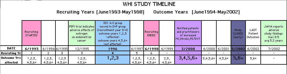
Objective: Perform a statistical analysis of time dependence on the published Mortality Rates from a carefully designed hormone study of daily estrogen (conjugated equine estrogen 0.625mg- CEE) plus progestin (medroxyprogesterone acetate 2.5mg- MPA).

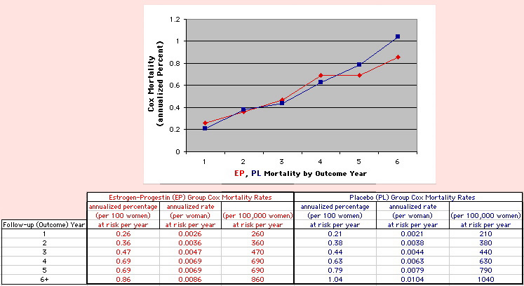
Design: The Annualized Cox Mortality Hazard Rates in the Estrogen/Progestin-

Treatment(EP) and Placebo(PL) Groups from the published data of the Womens Health Initiative Study [JAMA, July 17, 2002, 288(3):p321-333] are fit using a Least Squares Linear Regression Model for a single Predictor (Hormone Treatment Group) and a single Outcome (Mortality) by Outcome Year, and between-Group slope and intercept differences are obtained.

A Student T-Test on the slopes and intercepts of the binary rate data fits, and a Two-

Sample T-test on the differences are used as tests of significance.

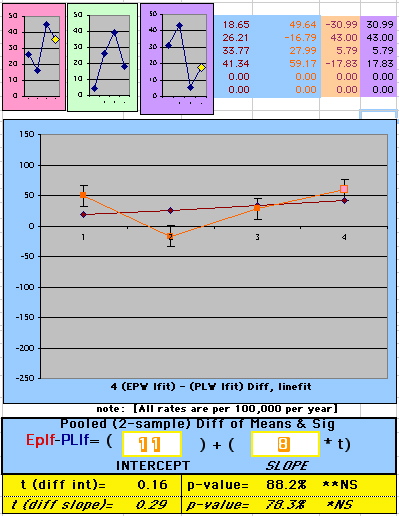
Results: The groups have unweighted linear approximations to the Annualized Mortality Rates (intercept + slope*t) of EP=(136+120*t) and PL=(26+159*t) deaths per 100,000 women at risk per year respectively, where t is the Outcome Year (1 to 6+ years, average 5.2 years). The EP intercept [CI=11to261], EP slope [CI=88to152] and PL slope [CI=126to192] obtained are significant [p<0.04], and the PL intercept [CI=-104to156] is not significant [p=0.6] from 0 by Student T-test using the sample estimates of mean and variance (T=2.78, 4df, 95%CI).

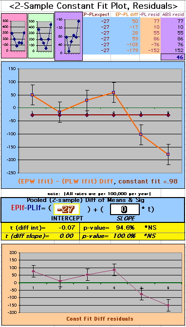
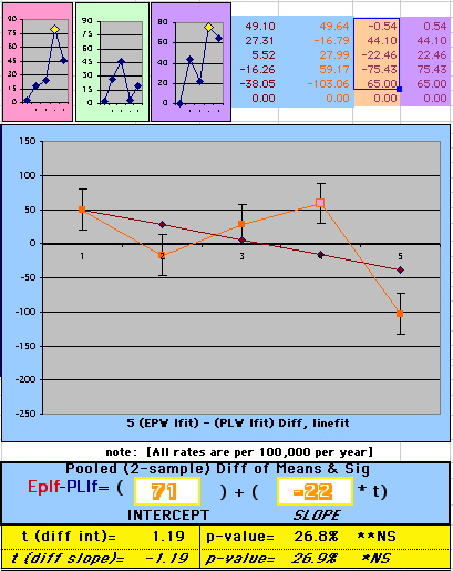
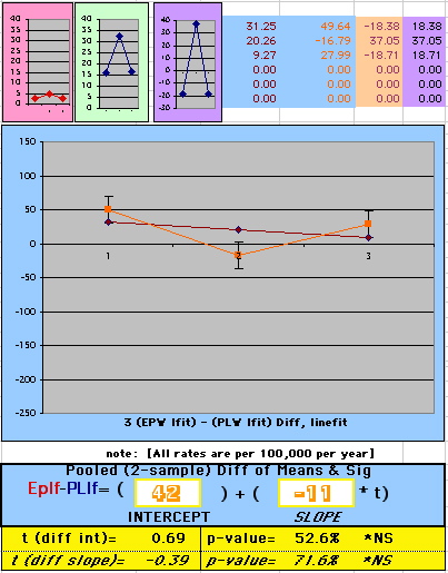
The Overall Mortality Rate Difference (OMRD)= EP-PL=(110-39*t) deaths per 100,000 women at risk per year. The slope difference is significant [CI=-76to-2, p=.04], while the intercept difference is not significant [CI=-35to255, p=.12] from 0 by Two-Sample T-test between the Groups (T=2.23, 10df, 95%CI).

Conclusion: A statistical analysis of time-dependence on the published Mortality data from the Womens Health Initiative Study is performed, consistent with a time-dependent decrease in Mortality between the Estrogen/Progestin(EP) and Placebo(PL) groups.(c)


DATA SOURCE

The Annualized Cox Mortality Rates from the Women's Health Initiative Study (WHI 2002)1 are reproduced here:


RESULTS OF ANALYSIS

This analysis uses the Least Squares method, which finds the linefit that minimizes the sum of the squared vertical distances between the actual data(y) and predicted fit(Y) values over time. This is done for each study group. (See the discussion of statistics and D&T [13 p195]).


The Annualized Cox Mortality Least Squares Rate Fits obtained by Year for the
Prempro Estrogen-Progestin (EP) and Placebo (PL) Groups are:

rate at year 0
INTERCEPT
rate increase each year
SLOPE
Estrogen-Progestin Group
136
26
120
159
Deaths per 100,000 women at risk per year
Placebo Group
The Straight Line Fits (EP pink line & gold text , PL pink line & pink text ) to the
Cox Rates (dkblue line and text) are shown here, with the
Residuals [Data-Expected] (brown text , shaded in cream).
Because the event rates are low, the data are well approximated by a straight line. Note, however, a large deviation from a straight line fit for Year4 in the EP group (pink diamond).


The EP, PL data and Linefits are shown directly below (left) next to the Difference between the Mortality Rate Intercepts and Slopes from the Linefits (right). The WHI Mortality Fits are re-shown below that graphed against each other, again next to the Difference Fits. Significance estimates for the Linefits using Student's T-test for Least Squares are shown there for EP (shaded in pink) and PL (shaded in paleblue).The Annualized Mortality Rates are shaded in purple, the Linefits are shaded in grey, and the (Data-Expected) Residuals from the Linefits are shaded in cream for these. .

The time dependent Overall Mortality Rate Difference Fit (OMRD),
EP-PL = Intercept - Slope * [Time] is:

OMRD = EP-PL = 110 - 39 * [Outcome Year]
Deaths per 100,000 women at risk per year


The EP-PL Difference is shaded in ltblue. The Difference in the Mortality Rate Fits is (110) in Year0, and decreases by (-39) each year, deaths per 100,000 women at risk per year. The Residuals of the Difference (Data minus Expected) are shaded in tan. Significance estimates for difference using the the Two-Sample Student T-Test and Probabilities is highlighted in yellow (or green if significant at 5%).
Note: The Absolute Value of the Residuals are listed top right of the 2-Sample Difference graph. EP Abs(Residuals) are shaded in pink, PL Abs(Residuals) are shaded in pale blue, and the Absolute Value of the Difference of the Residuals |EP-PL| are shaded in purple.
[click images to enlarge]

WHI MORTALITY FITS
WHI MORTALITY DIFFERENCE FIT
Timothy Bilash MD OBGYN www.DrTimDelivers.com 10.2004


If two groups have the same mortality rates, then the OMRD Difference plot would be expected on average to have a zero Slope and a zero Intercept ( ltblue shading above). A decreasing slope is found, however. Again note the large Residual for Outcome Year4.


This analysis utilizes the DIFFERENCE, while the WHI reported the RATIO of the Hormone and Placebo Annualized Hazard Rates. Because event rates are low, ratio and difference plots versus time have the same shape. The Ratios of the WHI Cox Annualized Rates by Year (EP/PL in red) are plotted below with the published overall constant Hazard Ratio of HR=.98 (grey line).[1]


To compare our Least Squares Difference Fit to the published WHI Hazard Ratio (presuming a constant Hazard Ratio or zero difference slope), Least Squares Linefits to the Annual Cox Rates (LS) are calculated assuming equal rate-slopes. The Cox Mortality Rates Data Difference (
orange line) and the Least Square Constant Difference Linefit obtained (brown line = constant = -27, zero slope obtained because of assumption of equal slopes) is shown at left. Note that the Residuals for the restricted Constant Difference (purple text, shaded in tan) are larger compared to the unrestricted LS Difference Linefit shown again at right below. They Residuals also do not appear randomly distributed about zero when comparing the Plots of the Residuals (shaded in tan).

Difference EP-PL / Constant Slope Linefit
Difference EP-PL / Unrestricted Slope Linefit


DISCUSSION OF LEAST SQUARE ANALYSIS

The Least Square analysis is equivalent to a weighted mean of the data, and as such is dominated by any outliers (extreme data points). Note the the largest Residuals are in Year4 for EP and Year3 for PL. Techniques such as the Percent Trimmed Mean, Least Trimmed Squares (called Least Trim Squares here to help distinguish from the Trimmed Mean) and M-estimators can greatly improve the accuracy of the means and variances, particulary for the means.

A modification of the Least Trim Squares (LTS) method [17 p212] is shown here for illustration. The Least Trim Squares essentially removes the contribution of up to 50% of the points with greatest deviations from the Linefit. Here the greatest deviation in each group is excluded (data points in
cream text with purple shading), and the Slope and Intercept differences calculated as for the Least Squares before. The LTS is excellent in many cases for improving the estimate of means (Slope and Intercept values). The improvement seen in the significance (SE and CI), however is not as great as indicated here, because the SE for the LTS is estimated using a non-rigorous method. The LTS Mean is more reliable than the untrimmed with this method for a wide range of distributions.

There is some change in the Intercept, but essentially no change in the Slope estimate with this Least Trim Square analysis. Note also the large Residual for Year4 (EP) and Year3 (PL).

[clic images to enlarge]


To further explore the time dependence of the difference data, later years are excluded (truncated) to obtain fits from the first- 3, 4, 5, and all data years shown below. There is a more negative slope difference and more positive intercept difference as more years are included, both differences increasing in magnitude. [Note that a Trimmed Mean is used for the first- 4 year graph only (2nd from the left below) - see 4 Year Effect of Trim below].

[click to enlarge]

The Slope of the Simple LS Linefit truncating the last 2 years (using the first four years left below) has a different sign (positive, not negative) than truncating the last 0, 1 or 3 years (using first 6, 5 or 3 years). Using the Trimmed Mean [17 p141], the Difference Slope and Intercept Residuals are improved (SE for the EP slope is dramatically decreased). This Trimmed fit is what is used for the last-2-year truncation in the multi-plot comparison above for better illustration, since this is highly dependent on the data point for Year 4 (right graph below and 2nd left above).


A table summarizing these modified fits is shown below. Although the Standard Error (SE) estimate for the Least Trim Square is not rigorously calculated, the Mean estimates are more reliable, and combining it with the Truncated Analysis provides a suggestion that Outcome Year4 (and perhaps Outcome Year3) differentially contributes errors to the SE beyond the expected random behavior, affecting the Mean Slope and Intercept values themselves less.


DISCUSSION OF LEAST SQUARE RESULTS FOR WHI

This leads to a search for possible explanations for the Outcome Year4 residual (affecting the EP and thus Difference and Ratio results).

Non-uniform Jump in Censored Patients at Outcome Year4

As noted in the 2002 paper, the number of censored patients exceeded the study design expectations. No discussion of how this might affect the results has been offered to date. In fact, adjusting just for a large number of censored patients is a problem. If in addition the differences between the groups or the number of censored patients is not uniform over time, it is not entirely clear how the analysis would be affected. [13 p240]

Below is an illustration of the Censored patients in the Kaplan-Meier Mortality Analysis from the WHI E+P Study. Note that there is a discrete jump in the censored patients for both groups at Outcome Year4, exactly the Year that displays a large Residual for EP. Initial Outcome Years 1,2,3 have a change in censor rate of about 0% per year [(+/-)1% for the EP group and essentially 0% for placebo group]. Later Outcome Years 4 and beyond have a change in censor rate of about (+)15% per year.a Because Outcome Year4 is a transition between the two censor rates, a larger Variance(Residual) for the Censored Outcome might be obtained relative to the other years, with less effect on the value itself. (The %changes data has been added for this Web version. Further results pertaining to the Censored patients will be added as soon as possible.)


Recruiting/Exposure not Coincident with Outcomes for Survival Analysis

Analysis of Survival is different from a true experiment in many ways. One is that Exposure is started at different times. Also Exposures and Outcomes are separated in time, with unequal time intervals.

Below is an illustration of the Recruiting and Outcome Groups that make up the Cox Analysis in the WHI. There are in effect 5 cohorts of patients, one for each year of recruitment, whose Outcome Years are shifted in chronological time. That is, Outcome Year4 is 96-97 for the patients recruited in 93-94, while Outcome Year4 is 99-00 for the patients recruited in 96-97.*b

WHI COX Outcome Years for each Recruiting Year Cohort


The Outcomes Groups in the Cox Analysis are made by combining the different chronological years that correspond to the same Outcome Year (Kaplan-Meier is different in this regard). Below is an illustration of this using the color scheme from the last graph.

Calendar Years comprising each WHI Cox Outcome Year


Events that have a non-uniform effect on recruiting, exposure, outcome diagnosis, or censoring over the time course of the study that can have anomalous effects on the outcome rates and comparisons of rates, if they differentially affect one group only.

Two identified events in the WHI are 1) the switching of patients from the Estrogen Only Study into the Combined Estrogen-Progestin Study in 1996 (patient hormone treatments were changed from E to E+P when this was done and patients included in the E+P Group for Outcome results), and 2) the announcement of increased risks in the Prempro Group in 2000. These moments are indicated on the recruiting graph above and in the general Timeline of the Study below. Further discussion of this will be added as soon as possible.


DISCUSSION OF THE WHI PUBLISHED MORTALITY RESULTS

Mortality is an extremely important clinical Outcome with a very clear clinical endpoint compared to other Outcomes. This paper examines the Annualized Cox Mortality Outcome data from the WHI (JAMA, July 17, 2002 [1]) over time. The individual patient data has not been released by the study yet (10/2004).

Cancer events are the major contributor to Mortality in the WHI study (47% =195/416). Coronary events are the other major contributor (29% =120/416). Note that the WHI reported no statistically significant increase in Coronary Heart Disease Mortality or Total Mortality with the use of continuous Prempro.[2,3,4,5,6,7,8]

The WHI study was publicized as a "carefully designed hormone study" concluding that continuous oral Estrogen/Progestin Hormone Treatment (Prempro CEE.625/MPA2.5) "should not be initiated or continued for primary prevention" of Coronary Heart Disease.

However, numerous problems in the study, such as high treatment crossover and dropout rates, have clouded the Outcome results, which conflict with other studies.[7,9] It can be argued that although the selection of exposure group was randomized, the actual exposure to hormone itself was not well controlled.

Many publications, societies and government agencies have echoed the conclusions of the study without examining the study shortcomings.[10,11,12] This paper is an attempt to look at the conclusions about Mortality.


STATISTICAL COMMENTS

Analysis of Survival Data requires a compound outcome to deal with the problems of analyzing the data before all events have actually happened. Ideally, one would wait until all patients die to do the analysis, which is not practical. So time and events get lumped together as one Outcome Statistic (events per time to event for the Hazard Function, or some variable like person-years). An early or late timing of diagnosis for the same number of events can have the same effect as a change in the number events at the same timing.

Considerable bias can occur with Survival Analysis [13 p217]
if the time intervals are large (not a problem with Kaplan-Meier)
if many withdrawals occur
if withdrawals do not happen on average midway in the interval (Cox Hazard Model or Kaplan-Meier)

Unfortunately, "little information is available to guide investigators in deciding which statistical analysis is appropriate for any given application of Survival Analysis, and research on biostatistical methods for analyzing survival data is still underway." [13 p224]


STUDY FACTORS THAT AFFECT THE ACCURACY OF THE WHI STUDY

Cross-overs
Dropouts
Contamination of Exposure
Censoring
Unblinding
Early termination, decreasing the statistical accuracy of any time-dependent analysis done on survival data.[21]


USE OF THE STUDENT T-TEST FOR RATE DATA

A proportion is a special case of a mean of 1's and 0's: the mean is simply the proportion itself. Student's T-Test on proportions is thus equivalent to an analysis on the means of binary rate data, and can be used as a test of significance for binary rates. [13 p108; 15] The Student T-Test is used here as a measure of significance for the Least Squares Fits.

A Two-Sample Independent Groups T-Test can be used to ask whether the means of two groups are equal when observations are numerical (continuous or means, ratios or proportions). [13 p133] Provided that the exposure risk is randomized, the Two-Sample T-Test is a valid approximation to the exact randomization experiment, free of the random sampling assumption or the assumption of exact normality. [14 p95]

Limitations of the T-test for significance of means relates primarily to missing an actual difference (beta error, low power =1-beta) rather than finding a difference when there is none (alpha error), particularly if the distributions have the same shape. [16;17 p107,120;18]


STATISTICAL FACTORS THAT AFFECT THE ACCURACY OF THE STUDENT T-TEST

Non-identical Population Distributions
(shape)
Non-constant Population Variances
Non-random samples
Correlation of Outcome with other factors (time of event)
Unequal Sample Sizes
Non-normal population distributions (see below)


STATISTICAL CALCULATIONS (see Dawson and Trapp [13])

Definitions and Least Square Equations: (p195)
x,y are the Sample Means
x is the Predictor (independent) Sample Mean value
y is the Outcome (dependent) Sample Mean value
YE=Y,XE=X are the Expected Sample Means
XE is the expected x Sample Mean for the Sample (x,y)
YE = Y= a+bx is the expected y Sample Mean for Sample (x,y)
Y= a+bx = YE is the regression line fit
y-YE = e = error term = residual
y=[a+bx]+e=Y+e
•n is the number of samples
•xbar,ybar are the Grand Sample Means
xbar = SUM(x)/n
ybar = SUM(y)/n
b=SUM[(x-xbar)(y-ybar)]/ SUM[(x-xbar)2] = Slope of the Linefit
a=ybar-b*(xbar) = Intercept of the Linefit

Assumptions
for the least squares fit (p197, 201)
•y is normally distributed about its expected value Y
•the expected values Y form a straight line
•the expected values Y are independent
•Variance of y is constant for every x
ybar (the mean of sample y's) = µ (mean of the population distribution)
•regression is a robust procedure and may be used in many situations in which the assumptions are not met, as long as the measurements are fairly reliable and the correct regression model is used
•if regression equations are calculated blindly without examining plots of the data, investigators can miss very strong but nonlinear relationships


One-Sample T-Test for Slope and Intercept (p196-201, 238)
want to perform a separate statistical test on slope and intercept obtained from Least Square Linefit
The T-Test can be used to determine whether Least Square regression coefficients are non-zero and to form confidence intervals, using the Standard Estimate of the Error (SE)
SE = Sqrt(SUM[(y-ybar)2/(n-2)]) = (Standard Deviation=SD)/Sqrt(n)
b0 = expected Intercept (= 0 for zero Intercept)
T(Intercept) = {a-b0} / {SE*Sqrt[(1/n)+[xbar2/SUM(x-xbar)2]}
denominator of this = SE(Int) = Standard Error of the Intercept
T(Slope) = SE2/[SUM(x-xbar)2]


Two-Sample T-Test for Differences (p135,139)
•significance for difference of means between two sample groups
assume random sampling (Student/Gossett)
assume equal Population Variances
T = (y1bar-y2bar) / Sqrt[SDp2(1/n1 + 1/n2)]
y1bar,y2bar is the sample means of group 1&2
n1,n2 is the sample sizes
SD1,SD2 is the sample variances
the assumed estimate of the common population variance is
SDp2 = [(n1-1)SD12 +(n2-1)SD22] / [n1+n2-2]
SE12, SE22 = SD12/n1, SD22/n2

SDp2 = [(n1-1)SE12/n1 +(n2-1)SE22/n2] / [n1+n2-2]
SE2(Difference)=SE2=SDp2(1/n1+1/n2)
SE2=SE12+SE22

Note: here SE is the pooled SE for the difference (SEE) , not to be confused with the SE for one sample. In this poster for convenience, SE is used for both the one sample and difference calculations, and should be clear from context.

Assumptions
for 2-Sample T-Test (p137-138)
each group follows a normal distribution
each group is independent
each group has the same population variance
however, with equal sample sizes, this requirement can be ignored (the 2-sample T-Test is robust with equal sample sizes)


REFERENCES

[1]
"Risks and Benefits of Estrogen Plus Progestin in Healthy Postmenopausal Women", Writing Group for the Women's Health Initiative Investigators, JAMA, July 17, 2002, 288(3):p321-337
[2] "Estrogen and Progestin and the Risk of Coronary Heart Disease", Manson JE et al, NEJM, 349:p523-534
[3] "Influence of Estrogen Plus Progestin on Breast Cancer and Mammography in Healthy Postmenopausal Women", Chlebowski RC et al, JAMA, 2003;289:3243-3253
[4] "WHI: Now that the dust has settled, Creasman WT, Hoel D and DiSaia PJ, Am J Obstet Gynecol, Sept 2003, p621-626
[5] "Cardiovascular Disease and Postmenopausal Hormone Therapy", Speroff L, Current Controversies in Obstetrics and Gynecology, Nov22-24 (2002) Newport Beach, CA
[6] "Postmenopausal Hormone Therapy and Breast Cancer", Speroff L, Current Controversies in Obstetrics and Gynecology, Nov22-24 (2002) Newport Beach, CA
[7] "The randomized world is not without its imperfections: reflections on the Women's Health Initiative Study, McDonough PG, Fertility and Sterility, 78(5), November 2002, p951-956
[8] "Results from the Women's Health Initiative", Bilash T, August/October, 2002 [www.DrTimDelivers.com]
[9] "Hormonal Therapy Following Breast Cancer", Wren BG, in Proceedings of the Second International Symposium of the Portugese Menopausal Society 1999, p55-56
[10] "Preliminary Statement to ACOG Membership on the Women's Health Initiative Study", July 10, 2002
[11] "FDA Approves New Labels for Estrogen and Estrogen with Progestin Therapies for Postmenopausal Women Following Review of Women's Health Initiative Data", January 8, 2003
[12] "New Federal Report on Carcinogens Lists Estrogen Therapy, Ultraviolet, Wood Dust", NIEHS PR#02-11, NIH, December 11, 2002
[13] Dawson B, and Trapp R, Basic Clinical Biostatistics (2001)
[14] Box , Hunter and Hunter, Statistics for Experimenters (1978), p507
[15] Colton T, Statistics in Medicine (1974), p35
[16] Bowers D, Medical Statistics from Scratch (2002), p42,131
[17] Wilcox R, Fundamentals of Modern Statistical Methods (2001)
[18] Colton T, Statistics in Medicine (1974), p82,108
[19] Koosis D, Statistics (1985), p139
[20] Bilash, T [unpublished]
[21] van Belle, G, Statistical Rules of Thumb (2002), p72


Special Thanks
to Rand R. Wilcox for his generous expert opinions about the Least Trimmed Squares and Bootstrap statistical techniques.


Timothy D. Bilash MD OBGYN 10.2004

(a) censored patients paragraph and graph revised 02.16.05
(b) outcome groups paragraph refined and graphs revised 03.01.05
(c) original abstract used the word difference in mortality, decrease is more accurate statement 01.01.08

__________________________________________________________

This poster is Dedicated in Memory of
Peg Harris, Ruth Howard and Helen Kolesnik Bilash

__________________________________________________________


goto homepage


page views since Oct2004